California Housing Prices

Python Notebook (Google Colab)

CaliforniaHousingPrices.ipynb

---

Introduction

Objective

Using a famous dataset on Kaggle, I will be using this flow to demonstrate how to create a regression-based machine learning model. Using the various attributes of the dataset, I will be showcasing the step-by-step process and thought process behind exploring the data, building the model, and validating the model.

Context

This is the dataset used in the second chapter of Aurélien Géron's recent book 'Hands-On Machine learning with Scikit-Learn and TensorFlow'. It serves as an excellent introduction to implementing machine learning algorithms because it requires rudimentary data cleaning, has an easily understandable list of variables and sits at an optimal size between being too toyish and too cumbersome.

The data contains information from the 1990 California census. So although it may not help you with predicting current housing prices like the Zillow Zestimate dataset, it does provide an accessible introductory dataset for teaching people about the basics of machine learning.

Data Dictionary

1. Longitude (float64): The longitude of the house
2. Latitude (float64): The latitude of the house
3. Housing Median Age (float64): The median age of the house
4. Total Rooms (float64): Total rooms of house
5. Total Bedrooms (float64): Total bedrooms of house
   • 207 (1.03%) missing values
6. Population (float64): Population of the area where house is in
7. Households (float64): The number of households in the area
8. Median Income (float64): The median income of the household
9. Median House Value (float64): The median house value ⇒ Target Variable
10. Ocean Proximity: If the house hold is near the ocean

Note: Median values are being treated as stated above. This may not be the true context of the data columns.

---

Exploratory Data Analysis

Basic Inspection of Dataframe

At the beginning of every data science project, I will read in the pertinent dataset(s) and do any preliminary sorting and selecting. In this instance, since we are using an external data set that we have not collected ourselves, we can simply read it into a dataframe and start analyzing the dataframe.

I do the following steps for every single dataframe that is read in. The dataframe is read into a variable df.

Shape of dataframe

# Shape of dataframe
df.shape

Columns of dataframe

# Columns of dataframe 
df.columns

Duplicated rows in dataframe

# Check for duplicated rows in the dataframe
df.duplicated().sum()

Top five rows of dataframe

# Head of dataframe
df.head()

Information on dataframe

# Information of dataframe
df.info()

Simple Null Value Count in each Column of dataframe

# Sum of null values in each column
df.isnull().sum()

Missing Numerical Summary of dataframe

# Get numerical summary of missing data by column
def missing_numerical_summary(df):
    total = df.shape[0]
    missing_columns = [col for col in df.columns if df[col].isnull().sum() > 0]
    missing_percent = {}
    for col in missing_columns:
        null_count = df[col].isnull().sum()
        per = (null_count/total) * 100
        missing_percent[col] = per
        print("{} : {} ({}%)".format(col, null_count, round(per, 3)))

# Get numerical data of missing values
missing_numerical_summary(df)

Describe numerical columns of dataframe

# Describe dataframe 
df.describe().T

From the process above, the following was discovered:

• There are 20,640 observations in the dataframe.
• There are 10 columns in the dataframe.
• The total_bedrooms column has 207 or 1.03% values missing.
• The numerical values do not seem to have any nonsensical values.

Univariate Analysis

The purpose of univariate analysis is to understand each column of data. For numerical columns, we want to understand the overall distribution. A histogram and a boxplot can be constructed to understand the interquartile range and the shape of the distribution.

Histogram-Boxplot Function

# Takes a dataframe and a numerical columns
# Returns a joint boxplot and histogram, prints mean and median values
def histogram_boxplot(data, feature, figsize=(12, 7), kde=False, bins=None):
    """
    Boxplot and histogram combined

    data: dataframe
    feature: dataframe column
    figsize: size of figure (default (12,7))
    kde: whether to show the density curve (default False)
    bins: number of bins for histogram (default None)
    """
    f2, (ax_box2, ax_hist2) = plt.subplots(
        nrows=2,  # Number of rows of the subplot grid= 2
        sharex=True,  # x-axis will be shared among all subplots
        gridspec_kw={"height_ratios": (0.25, 0.75)},
        figsize=figsize)  # creating the 2 subplots
    
    sns.boxplot(data=data, x=feature, ax=ax_box2, showmeans=True, color="violet")  # boxplot will be created and a star will indicate the mean value of the column
    
    if bins:
      sns.histplot(data=data, x=feature, kde=kde, ax=ax_hist2, bins=bins, palette="winter")
    else: 
      sns.histplot(data=data, x=feature, kde=kde, ax=ax_hist2)  # For histogram
    
    ax_hist2.axvline(data[feature].mean(), color="green", linestyle="--")  # Add mean to the histogram
    
    ax_hist2.axvline(data[feature].median(), color="black", linestyle="-")  # Add median to the histogram

    print("Mean: " + str(data[feature].mean()))
    print("Median: " + str(data[feature].median()))

Histogram of All Variables

df.hist(bins=60, figsize=(15,9), color='blue')
plt.show()

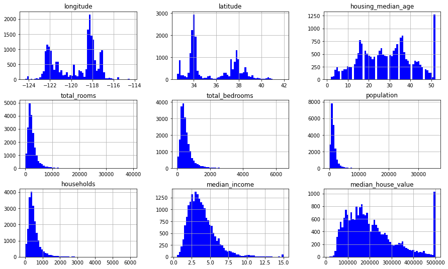
Longitude and latitude are technically numerical columns but it is best to not treat them as interval-ratio variables. Instead, we shall disregard them for the sake of the simple regression model.

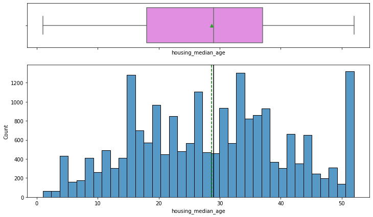
housing_median_age

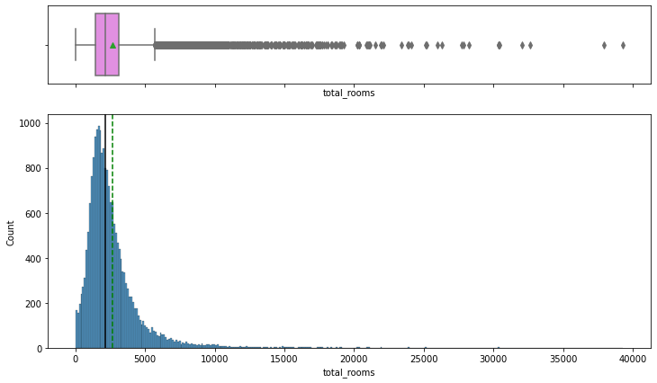
total_rooms

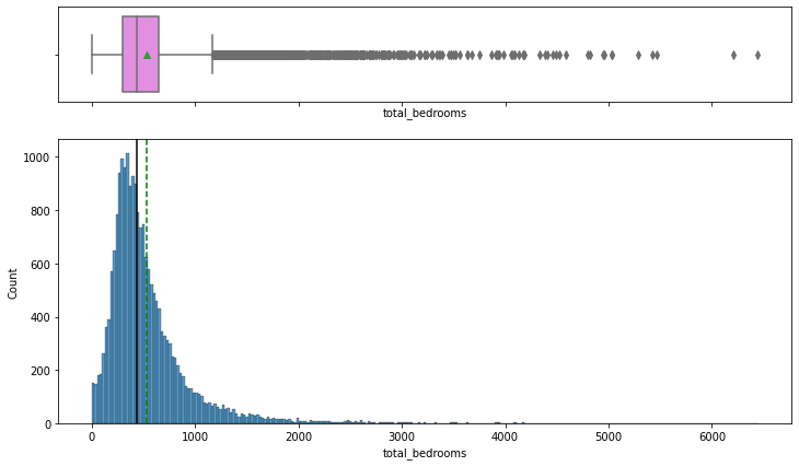
total_bedrooms

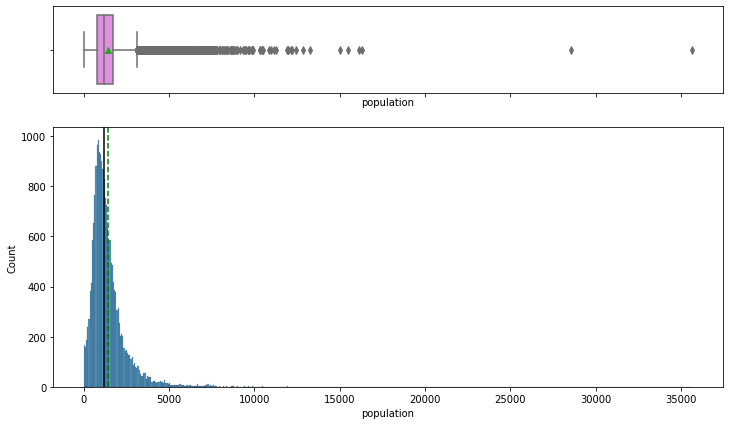
population

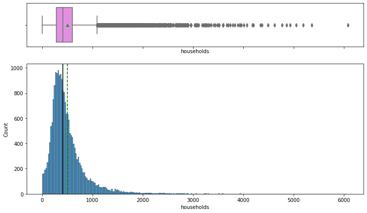
households

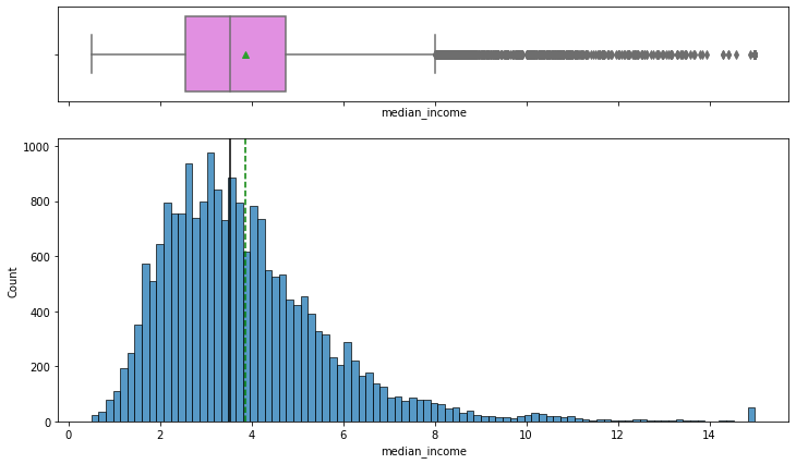
median_income

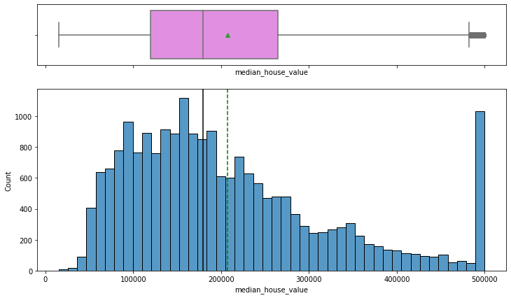
median_house_value

ocean_proximity

Value counts code

# Frequency 
df['ocean_proximity'].value_counts()

# Percentage
df['ocean_proximity'].value_counts(normalize=True).to_frame().style.format('{:.2%}')

Value	Frequency	Percentage
<1H OCEAN	9,136	44.26%
INLAND	6,551	31.74%
NEAR OCEAN	2,658	12.88%
NEAR BAY	2,290	11.09%
ISLAND	5	0.02%

Univariate Analysis Takeaways:

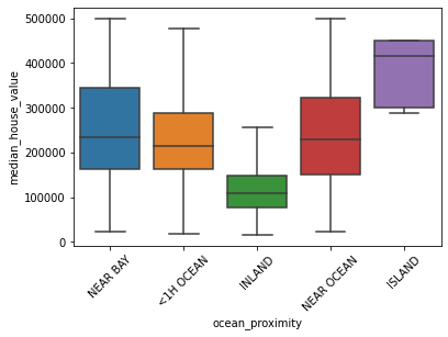
• housing_median_age is approximately evenly distributed, but has outliers to the right.
• total_rooms, total_bedrooms, population, and households are all positively skewed.
• median_income and median_house_value are also positively skewed but not extremely.
• median_income and median_house_value have outliers to the right.
• ocean_proximity will need to be divided into five Boolean columns.

Bivariate Analysis

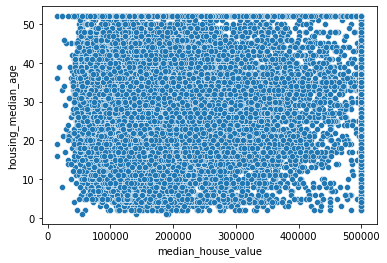
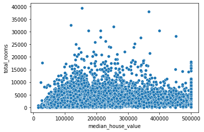
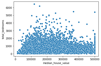
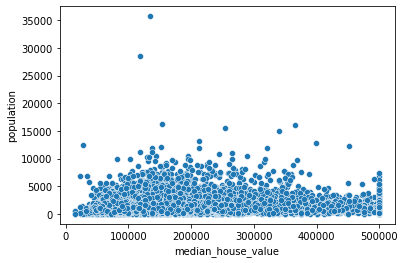
There are two main reasons for bivariate analysis: (1) to understand how independent variables correlate with the dependent variable, and (2) to understand if any of the independent variables correlate with one another.

median_house_value versus housing_median_age

median_house_value versus total_rooms

median_house_value versus total_bedrooms

median_house_value versus population

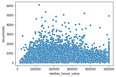
median_house_value versus households

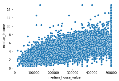
median_house_value versus median_income

median_house_value versus ocean_proximity

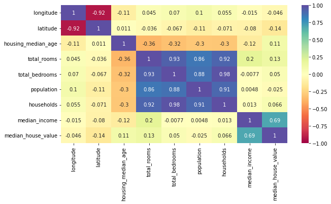
General Bivariate Correlations

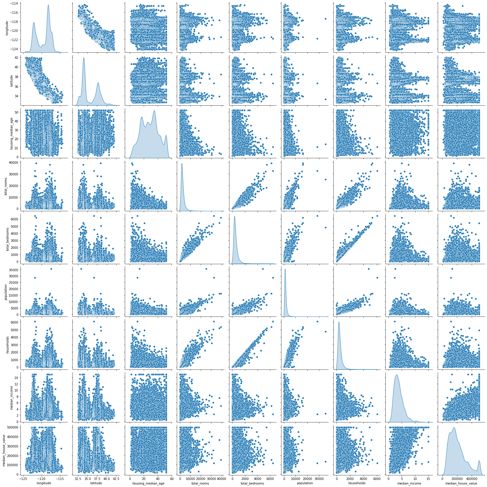
Bivariate Analysis Takeaways:

• median_house_value has a strong correlation with median_income.
• median_house_value does not have a strong correlation with any other variable.
• There is very strong correlation between total_rooms, total_bedrooms, population, and households. This strong correlation between independent variables should be dropped (by dropping all but one of these variables) due to multicollinearity problems.

---

Data Preprocessing

Missing Values, Handling, and Imputation

There are multiple ways to deal with missing values, here are some of them:

1. Drop the observations with missing values.
2. Drop the variables with missing values.
3. Impute missing values with the mean, median, or mode of the variable.
4. Impute missing values with the mean, median, or mode of a subset of the given variable.
5. Impute using an advanced method, such as imputing with a clustering algorithm (kNN imputation), or a tree-based model.

Since we have a very small portion of the data missing, a simple mean, median, or mode imputation will suffice. Ideally, we should identify the most appropriate measures of imputation and exhaust all options.

Since total_bedrooms are missing, we would want to impute the mean of that column using a subsect of variables with high correlation (total_rooms, population, and households). For this scenario, we shall impute missing values in the total_bedrooms and impute with a corresponding subsect of households (as they are very strongly correlated).

Code for imputing missing values in total_bedrooms using subsect of households

# imputing missing values in 'total_bedrooms'
df['total_bedrooms'] = df.groupby(['households'])['total_bedrooms'].transform(
    lambda x: x.fillna(x.mean())
)

Doing this resulted in 201 of the 207 missing values being imputed. But since we are left with 6 missing values, we shall impute in a very similar way but using total_rooms and population

Code for imputing missing values in total_bedrooms using subsect of total_rooms

# imputing missing values in 'total_bedrooms'
df['total_bedrooms'] = df.groupby(['total_rooms'])['total_bedrooms'].transform(
    lambda x: x.fillna(x.mean())
)

Code for imputing missing values in total_bedrooms using subsect of population

# imputing missing values in 'total_bedrooms'
df['total_bedrooms'] = df.groupby(['population'])['total_bedrooms'].transform(
    lambda x: x.fillna(x.mean())
)

By doing this we have been able to impute all missing values in total_bedrooms column.

Feature Engineering

Feature engineering is an essential part of the data science process as it allows for new data to be created from existing data. With our dataset, one important feature engineering that could be done is by taking longitude & latitude and creating city locations for each observation. These observations then could be used to create per-city Booleans. For the scope of this blog, we shall proceed by not doing any feature engineering. At a later time, testing out the effect of this feature engineering will be a great exercise.

Outlier Detection & Treatment

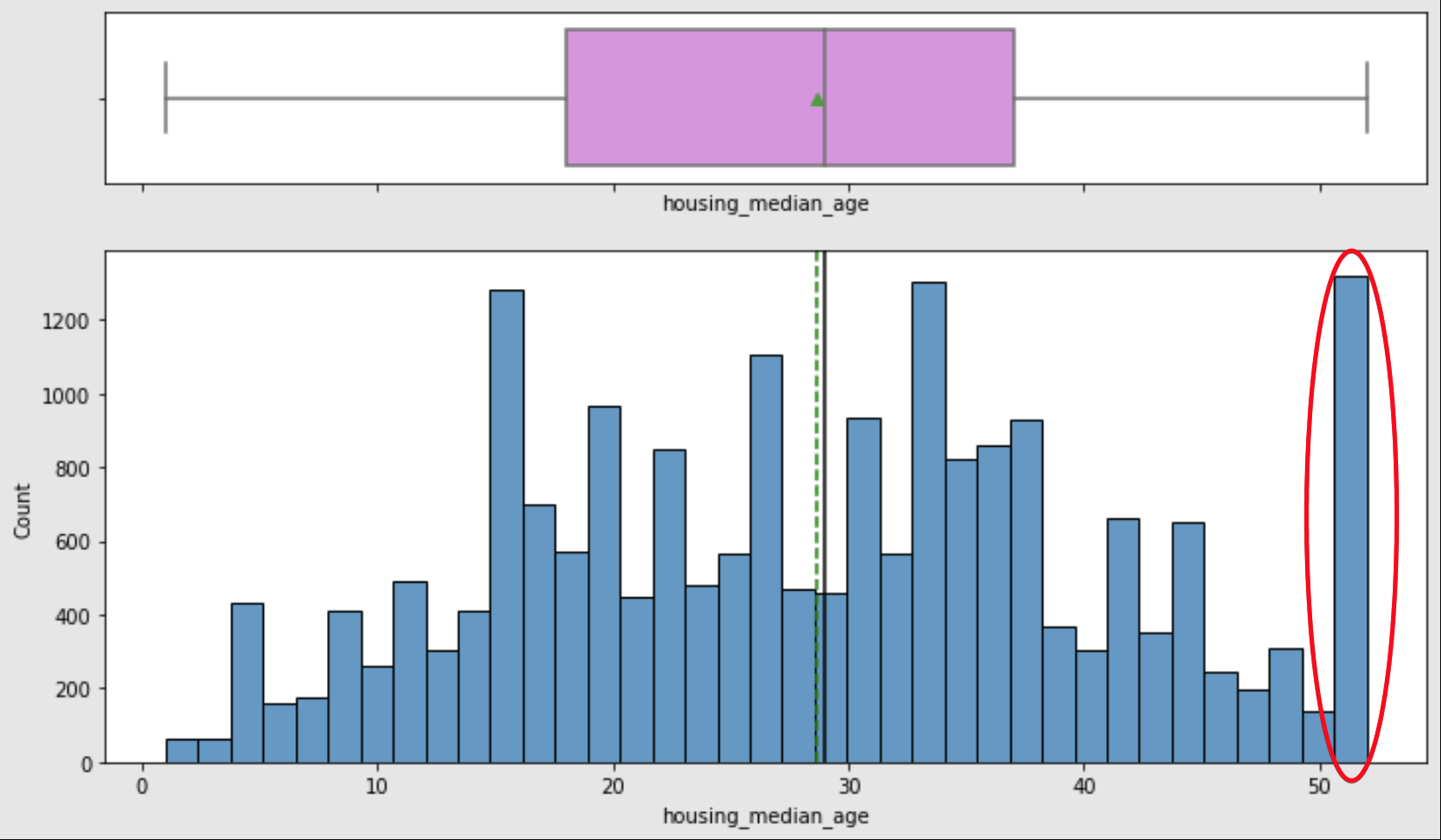
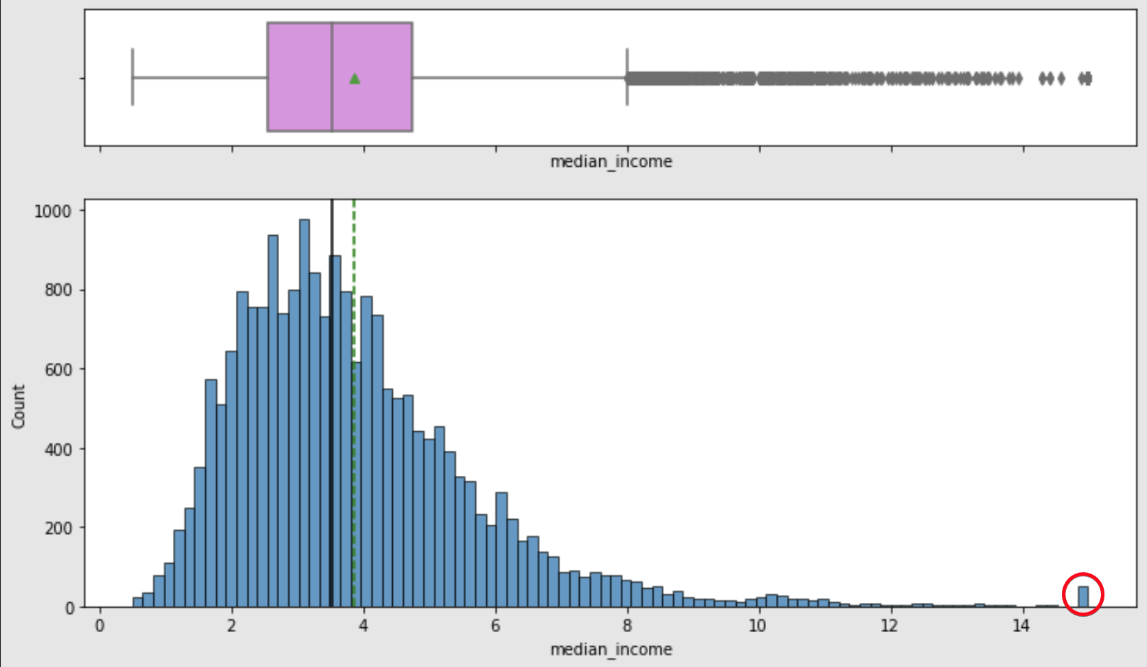
There are various ways to detect and treat outliers in data. In our case, we shall detect outliers by using the boxplots and histograms created in the Univariate Analysis section. housing_median_age, median_income, and median_house_value were all identified to have outliers to the right of their distributions.

housing_median_age Outliers

median_income Outliers

median_house_value Outliers

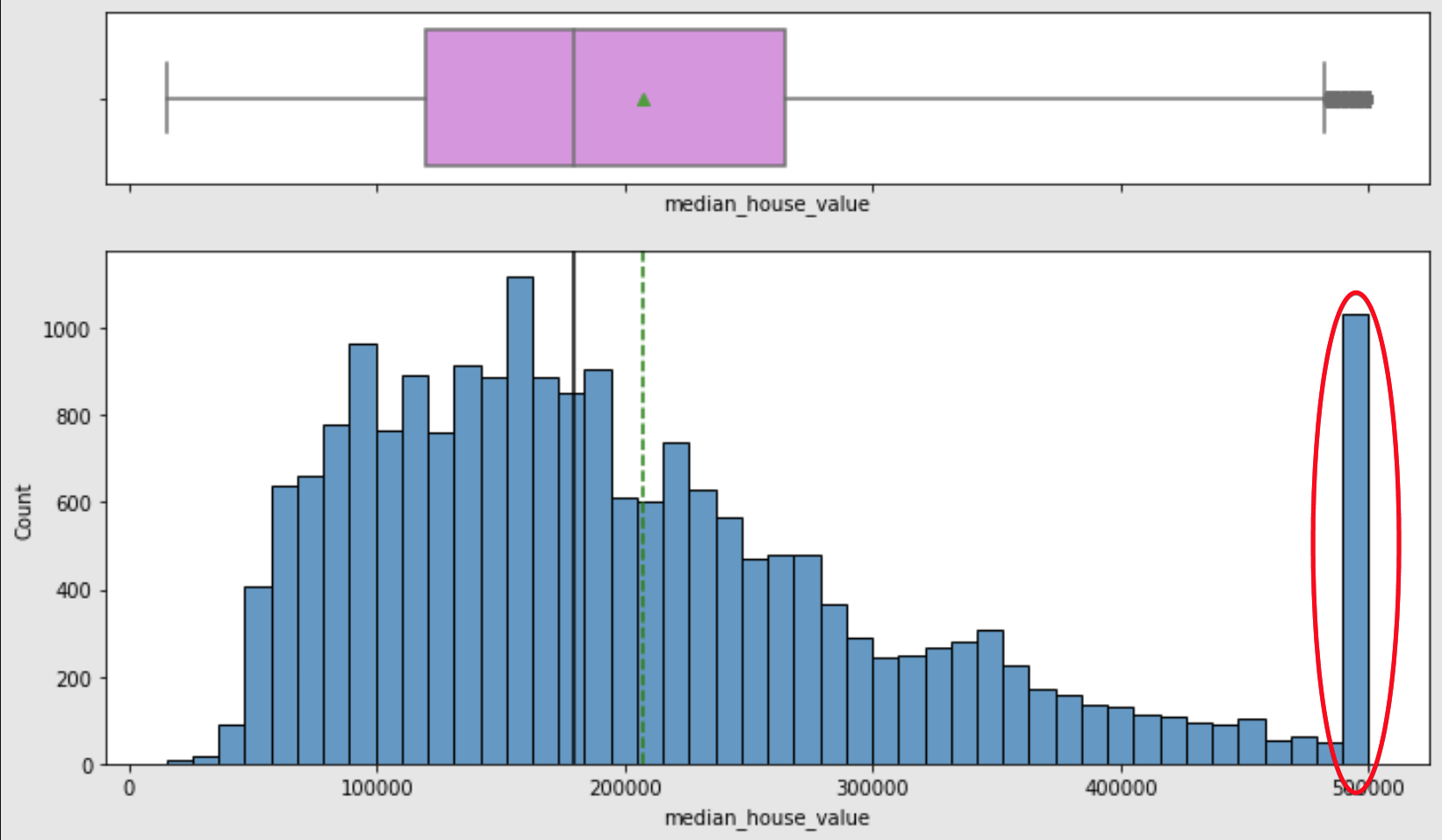
There are various methods to treat these outliers. First, if we believe the outliers are from human error or erroneous by some other factor, we can use an imputation methods to replace the independent variables' outliers. Second, if we believe the outliers are factual but are not representative of the model's use case, we are able to drop the observations of the outliers. Finally, if there are any outliers in the target (dependent) variable that does not help the model, this should always be dropped.

median_house_value Outlier Treatment

We want to treat median_house_value first because these observations will have to be dropped. As a result, other columns such as median_income and housing_median_age might also be inadvertently treated as well.

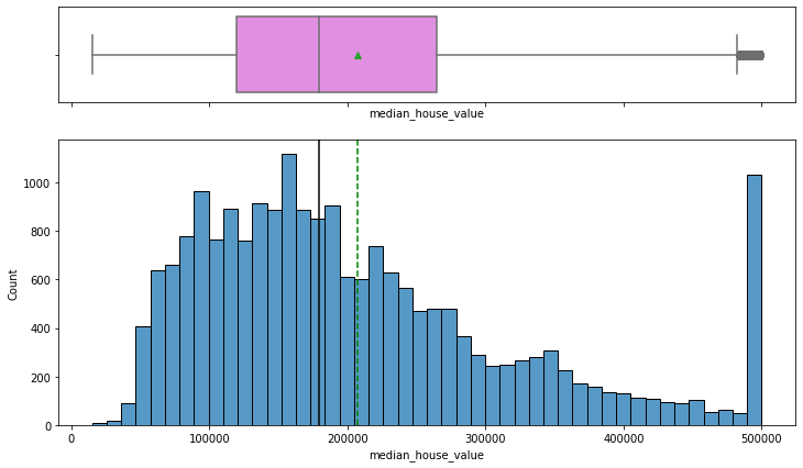
Taking a deeper look into values on the right side of the median household value's distribution, there are 965 rows that have an exact value of 500,001. Most likely, all of these houses exceeded $500,000 in value and therefore were categorized in this group. Since this data will most definitely bias our dataset, we shall drop these observations.

Before Outlier Treatment for median_house_value

After Outlier Treatment for median_house_value

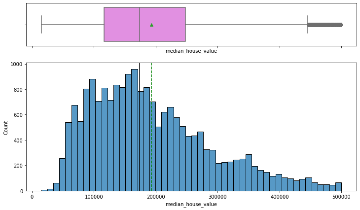
Through this treatment process, we have went from 20,640 observations to 19,675 observations.

median_income Outlier Treatment

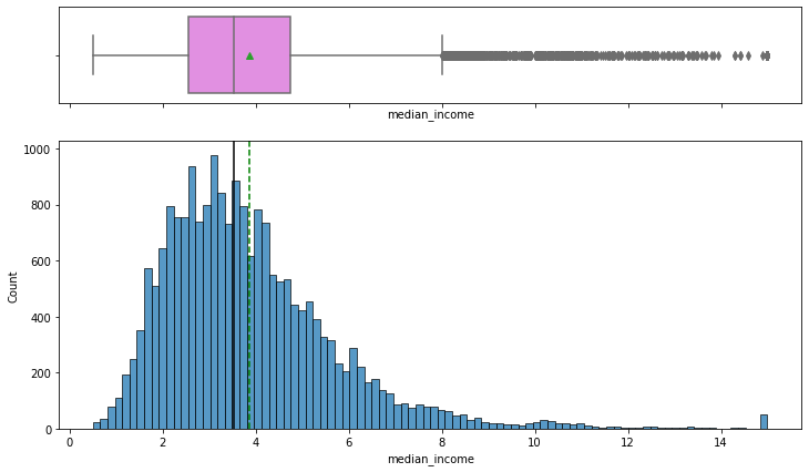
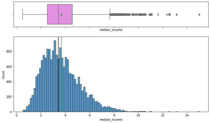
As suspected, the outliers in median_income were treated by treating outliers in median_house_value.

Before Outlier Treatment for median_house_value

After Outlier Treatment for median_house_value

housing_median_age Outlier Treatment

Unlike median_income, housing_median_age was not treated as a byproduct of treating outliers in median_house_value.

Before Outlier Treatment for median_house_value

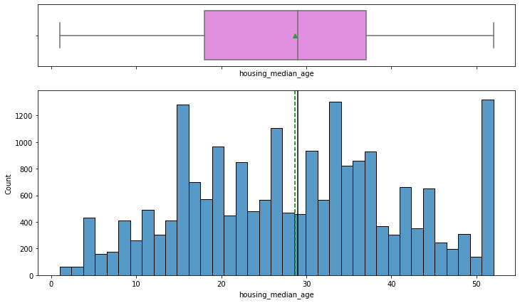
After Outlier Treatment for median_house_value

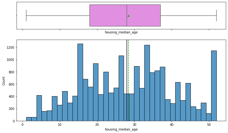
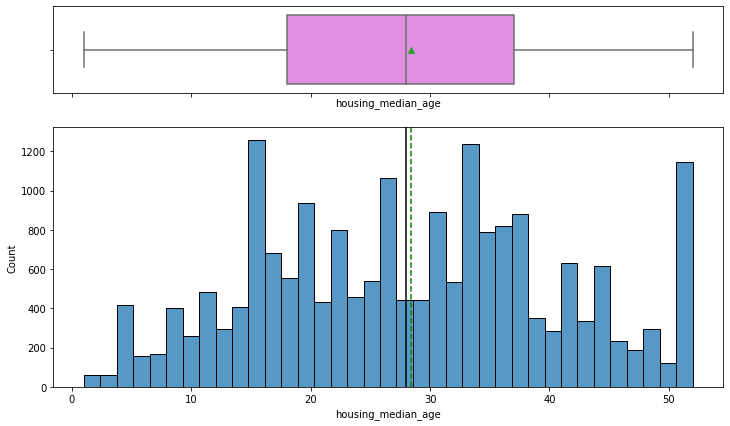
Taking a closer look, there are 1,103 rows that have an age of 52. Although some of these values are genuine, most of these values suffer the same capping that median_house_value did. Therefore, we shall approach this the same way and drop such values.

Before Outlier Treatment for housing_median_age

After Outlier Treatment for housing_median_age

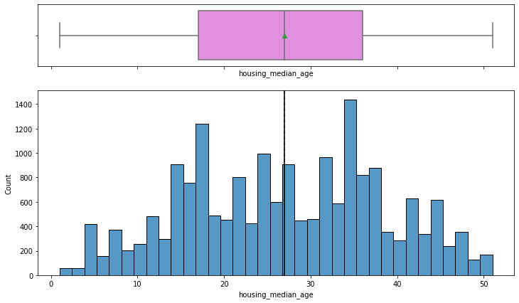
Through this treatment process, we have went from 19,675 observations to 18,572 observations.

Distribution Skew Treatment

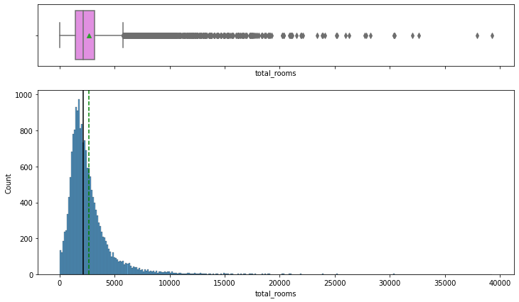
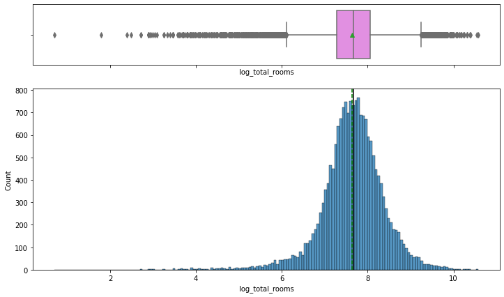
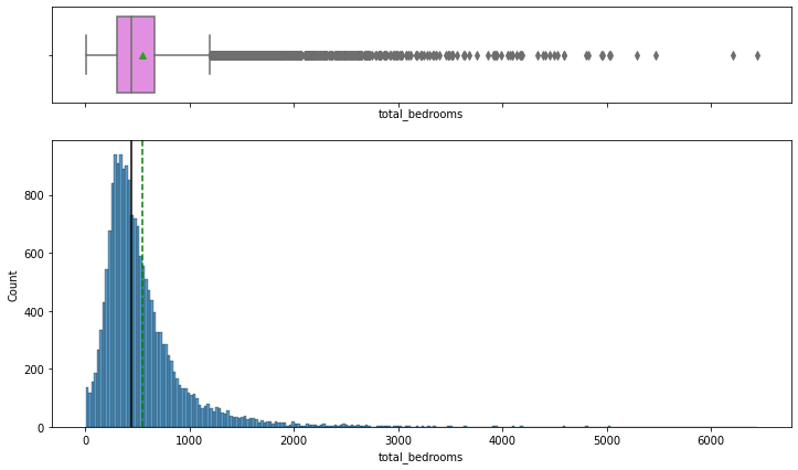
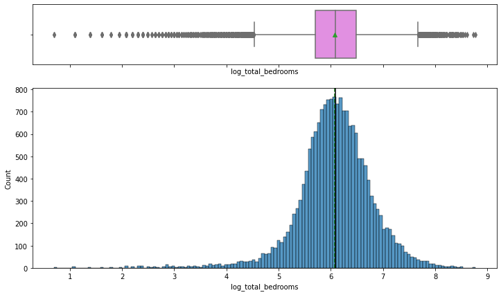
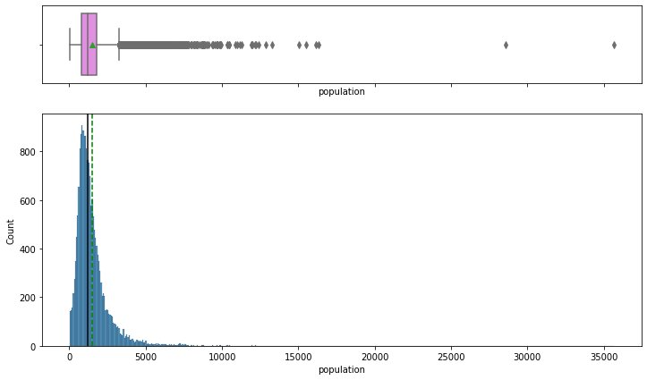
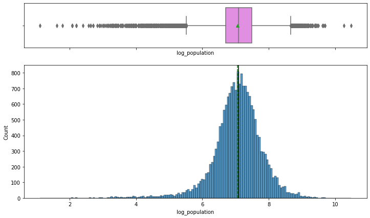
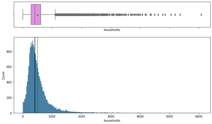
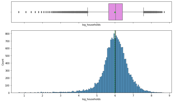
As found in the EDA process, total_rooms, total_bedrooms, population, and households are all positively skewed. All of these variables should be log-formatted in order to achieve an approximately even distribution, as this will help our model perform better.

total_rooms Log-Formatting

For this process we shall take the log of total_rooms and create a new column named log_total_rooms.

Before Log-Formatting total_rooms

After Log-Formatting total_rooms

total_bedrooms Log-Formatting

For this process we shall take the log of total_bedrooms and create a new column named log_total_bedrooms.

Before Log-Formatting total_bedrooms

After Log-Formatting total_bedrooms

population Log-Formatting

For this process we shall take the log of population and create a new column named log_population.

Before Log-Formatting population

After Log-Formatting population

households Log-Formatting

For this process we shall take the log of households and create a new column named log_households.

Before Log-Formatting households

After Log-Formatting households

Variable Standardization

For model performance, we shall use MinMaxScaler from the sklearn module to make each variable have an equal range. This will allow for each of the independent variables to have equal influence in the linear regression model. The dependent variable, median_house_value will be excluded so the validation metric is not biased. Similarly, median_income will also be untouched as it is not log-formatted and slightly skewed.

Code for Variable Standardization

# Standardize given variables using MinMaxScaler()
df3[['housing_median_range', 'log_total_rooms', 'log_total_bedrooms', 'log_population', 'log_households']] = MinMaxScaler().fit_transform(
    df3[['housing_median_range', 'log_total_rooms', 'log_total_bedrooms', 'log_population', 'log_households']]
)

Data Manipulation

There are various processes that fall under data manipulation, but in our scenario since linear regression only takes numerical values, we will need to alter the ocean_proximity column. Here, we shall take the the column and first change the column type to 'category'. Then, we shall create Boolean values for every single unique value for ocean_proximity except for one of them (to avoid multicollinearity problems).

Code for Creating Boolean Variables for ocean_proximity

# Create list of categorical columns
cat_vars = ['ocean_proximity']

# Loop through categorical columns and convert column type to 'category'
for colname in cat_vars:
    df3[colname] = df3[colname].astype('category')
    
# Create dummy variables for each column 
for colname in cat_vars: 
    df3 = pd.concat([df3.drop(colname, axis=1), pd.get_dummies(df3[colname], drop_first=True)], axis=1)

---

Model Building

Split Data into Train & Test

In order to avoid overfitting, we shall take a random sample (70%) of the data to train the linear regression model. Then, we shall test the built model with the remaining data to ensure we do not overfit the data. Usually there will be another withheld data set for final results but we do not have such data set available in our instance.

Code to Split Data

# Columns to drop from model building dataset
col_to_drop = ['longitude', 'latitude', 'housing_median_age', 'total_rooms', 
               'total_bedrooms', 'population', 'households']

# Select independent variables
X = df3.drop(col_to_drop, axis=1)

# Select dependent variable
y = df3[['median_house_value']]

# Split X and y into training and test set in 70:30 ratio
X_train, X_test, y_train, y_test = train_test_split(X, y, test_size=0.30, random_state=1)

Fit Linear Model

Now using the training datasets, we can train the linear regression model.

Code to Train Model

# Initiate linear regression model
regression_model = LinearRegression()

# Fit linear regression model to data
regression_model.fit(X_train, y_train)

Variable Coefficients

With a trained model, we can inspect the variable coefficients to see the effect of each variable. These are not very clearly interpretable as (1) some of the variables are log-formatted and normalized which make interpretation very difficult, and (2) we do not get any significance information as part of the coefficients.

Code to find Variable Coefficients

# Print coefficient for each variable for the linear regression model
for idx, col_name in enumerate(X_train.columns):
    print("The coefficient for {} is {}".format(col_name, regression_model.coef_[0][idx]))

# Print intercept for the linear regression model
intercept = regression_model.intercept_[0]
print("The intercept for our model is {}".format(intercept))

Variable	Coefficient
Median Income	43,032
Log Total Rooms	-632,151
Log Total Bedrooms	589,339
Log Population	-698,100
Log Households	540,753
INLAND (Boolean)	-63,113
ISLAND (Boolean)	258,915
NEAR BAY (Boolean)	-4,596
NEAR OCEAN (Boolean)	9,855
Intercept	188,440

One concerning observation is log_total_rooms, log_total_bedrooms, log_population, and log_households all have very large coefficients. This is usually due to multicollinearity problems. One solution is to take out three of the four variables and run the model again.

1st Model Validation through R² Values

Using the model we have just created we see the following R² values:

Sample	R² Value
Training Sample	0.6305
Test Sample	0.6062

With the current model, we are only able to explain 60.6% of the variance. We shall try dealing with the multicollinearity problem to see if that will improve our score.

Split Data, Train Model, & get Variable Coefficients for 2nd Model

Since total_rooms is the most highly correlated with our target variable, the other three variables (log_total_bedrooms, log_population, and log_households) will be dropped in an effort to combat multicollinearity issues.

Code to Split Data

# Columns to drop from model building dataset
col_to_drop = ['longitude', 'latitude', 'housing_median_age', 'total_rooms', 
               'log_total_bedrooms', 'log_population', 'log_households',
               'total_bedrooms', 'population', 'households', 'median_house_value']

# Select independent variables
X = df3.drop(col_to_drop, axis=1)

# Select dependent variable
y = df3[['median_house_value']]

# Split X and y into training and test set in 70:30 ratio
X_train, X_test, y_train, y_test = train_test_split(X, y, test_size=0.30, random_state=1)

Code to Train Model

# Initiate linear regression model
regression_model = LinearRegression()

# Fit linear regression model to data
regression_model.fit(X_train, y_train)

Code to find Variable Coefficients

# Print coefficient for each variable for the linear regression model
for idx, col_name in enumerate(X_train.columns):
    print("The coefficient for {} is {}".format(col_name, regression_model.coef_[0][idx]))

# Print intercept for the linear regression model
intercept = regression_model.intercept_[0]
print("The intercept for our model is {}".format(intercept))

Variable	Coefficient
Median Income	35,061
Log Total Rooms	52,720
INLAND (Boolean)	-71,117
ISLAND (Boolean)	293,731
NEAR BAY (Boolean)	3,435
NEAR OCEAN (Boolean)	16,383
Intercept	44,719

At a glance, these coefficients seemed to have fixed the multicollinearity issues as there are not "exploded" coefficient values. If the model performs better with R² values, then we can be sure that this is the correct decision.

2nd Model Validation through R² Values

Using the model we have just created we see the following R² values:

Sample	R² Value
Training Sample	0.5747
Test Sample	0.5640

With the second model, we are only able to explain 56.4% of the variance. This decrease in the model's ability the variance in data tells us that extra variables that were dropped are somewhat useful to the model. Therefore we shall revert to the first model and move forward.

Interaction Terms

Within a linear model, we are able to add in interaction terms between the independent variables to catch any interaction effects that might be occurring. While this will likely improve our R² values, this will also damage the adjusted R² value. The adjusted R² values takes into consideration how much each term contributes to model's ability to explain variance and penalizes terms that do not contribute to the model's ability to explain variance. We shall try creating interaction terms with 2 and 3 degrees (degrees refers to how many independent variables can be multiplied together in the linear equation).

Code to create Models with Interactions Terms (2 degrees)

# Initiate the PolynomialFeatures function, limit to two interacting terms
poly = PolynomialFeatures(degree=2, interaction_only=True)

# Create X_train set with interacting terms
X_train2 = poly.fit_transform(X_train)

# Create X_test set with interacting terms
X_test2 = poly.fit_transform(X_test)

# Initiate LinearRegression for polynomial regression model
poly_clf = linear_model.LinearRegression()

# Fit the polynomial regression model on train dataset
poly_clf.fit(X_train2, y_train)

# Predict price with polynomial test dataset
y_pred = poly_clf.predict(X_test2)

Code to create Models with Interactions Terms (3 degrees)

# Initiate the PolynomialFeatures function, limit to two interacting terms
poly3 = PolynomialFeatures(degree=3, interaction_only=True)

# Create X_train set with interacting terms
X_train3 = poly3.fit_transform(X_train)

# Create X_test set with interacting terms
X_test3 = poly3.fit_transform(X_test)

# Initiate LinearRegression for polynomial regression model
poly_clf = linear_model.LinearRegression()

# Fit the polynomial regression model on train dataset
poly_clf.fit(X_train3, y_train)

# Predict price with polynomial test dataset
y_pred = poly_clf.predict(X_test3)

Interaction Models Validation through R² Values

Model	Sample	R² Value
No Interaction Terms	Training Sample	0.6305
No Interaction Terms	Test Sample	0.6062
Two Degrees of Interaction Terms	Training Sample	0.6567
Two Degrees of Interaction Terms	Test Sample	0.6427
Three Degrees of Interaction Terms	Training Sample	0.6636
Three Degrees of Interaction Terms	Test Sample	0.6440

For both of the models with two & three degrees of interaction terms, the performed better than the previous model. Although this is the case, we should be aware of the exponential increase in terms in our linear equation:

Model	Terms
No Interaction Terms	9
Two Degrees of Interaction Terms	46
Three Degrees of Interaction Terms	130

---

Conclusion

By constructing a linear regression model with 3 degrees of interactions terms, we were able to explain 64.4% of the variance. It should be noted that this increase in R² value that comes from adding interaction terms comes at a cost of exponentially increasing the number of total terms in the linear equation. The selected model has 130 terms, whereas the initial linear regression model with no interaction terms only has 9 terms. This should be kept in mind when evaluating the model with other parameters such as adjusted R².

Future Steps

• Explore other regression machine learning models
• Explore feature engineering of the latitude and longitude variables